home

2DGI #1 - Global Illumination in Godot

Hello.

This is the first of a series of blog posts I plan to write, breaking apart the algorithms and implementation of a custom 2D global illumination (or path tracing, or radiosity, or whatever you want to call it) lighting engine in Godot.

To skip some preamble and get to the Godot implementation, click here. If you want to skip everything and get the code, click here.

I want to do more than just give you the code and tell you where to put it (after all, I’ve made the demo source available). Hopefully after reading through this, or even better, following along yourself, you’ll get a better understanding of the methods involved and be able to experiment and modify stuff yourself, to use in your own games.

Having said that, I will come clean and tell you I knew next to nothing about any of these subjects before around three months ago, so I am hardly the authority on the matter. However, around that time I did a lot of Googling and found smatterings of info and examples. The most useful resource was /u/toocanzs who wrote a shadertoy example of the technique (which was itself inspired by another reddit user’s example). It’s safe to say without this as a jumping-board my implementation wouldn’t exist. Apart from this, I only found a few other people who have done something similar - two of the more inspiring being Thomas Diewald’s animations and Andy Duboc’s images - but nothing with implementation details.

Come on get to the point I hear you cry, OK fine.

What’s The Point?

The point is that I’m lazy, and I want a lighting system that just works without me, the curator, having to worry about placing lights, probes, occlusion volumes, dealing with light blending, shadowing artifacts, yada yada, and what better way to achieve that than do it the way it just works in real life with actual rays of photons. Of course, I also want it to look amazing and unlike any other game out there. And I’ve looked, no other game I’ve found is doing this (probably because it’s really hard once you start building an actual game around it). Oh and it also needs to run well.

Tl;dr

• It needs to run well on medium spec hardware. No point in looking pretty if it makes the game unplayable.
• It needs to look good (bounced light, shadows, colour blending).
• It should make curation (i.e. levels, environments, content) easier, not harder, compared to more standard lighting techniques.

Looking At The Data

“The purpose of all programs, and all parts of those programs, is to transform data from one form to another.” - Jackie Chan, probably (actually I lied it was Mike Acton)

Let’s start by looking at the data we’re putting in, and the data we expect to get out the other end, so we can properly reason about the transform we need to do in the middle.

In - There are two entities we care about: Emitters and Occluders. We care about their position, rotation, shape, emissive (brightness) and colour for emitters, albedo (reflectivity) and colour for occluders.

Out - A brightness and colour value for each pixel in the scene, representing the amount of light gathered by that pixel from surrounding emissive surfaces.

We also need to consider the hardware (or platform) we’re running on. My goal when developing this technique was to eventually make a game that used it as a lighting engine, and the target platform would be PCs with medium-to-high spec graphics cards. This means we have access to the GPU and the potentially powerful parallel pixel processing proficiency (or PPPPPP, soundtrack to the amazing VVVVVV by Terry Cavanagh) it has, which we will utilise fully to transform our data from A to B.

Since the common data format of the GPU is the humble texture, we’ll be storing our input data in texture format. Thankfully it just so happens that most game engines come equipped with a simple method of storing spatial and colour information about 2D entities in texture data, it’s done by drawing a sprite to the screen! Well, that was easy, let’s move on to the fun stuff.

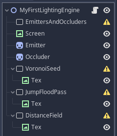
Setting The Scene

Ok, there’s an important thing we need to do first. By default, when you draw a sprite in most engines it will get drawn to the frame buffer, which is a texture (or a group of textures) onto which the whole scene is drawn, and then ‘presented’ to the screen. Instead we want to draw our sprite onto a texture we can then use as an input to our lighting shader. How to do this will differ depending on the engine or framework, I will show how it’s done in Godot.

Render Textures In Godot

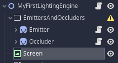
Godot has an object called a Viewport. Nodes (Sprites, Canvases, Particles, etc) are drawn to the closest parent Viewport, and each Scene has a root viewport even if you don’t add one manually, that root viewport is what presents it’s contents to the screen.

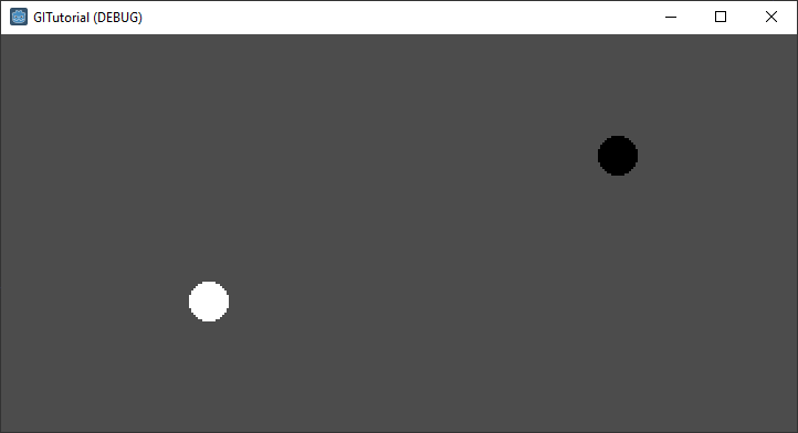
This means we can create a new viewport, add our emitters and occluders as child sprites to it, then access the resulting texture to feed into our lighting shader. Our sprites can be anything, but for now the emitter should be white and the occluder black.

I’m also going to create a TextureRect called Screen as a child of the root node. This will be how we display the contents of a viewport to screen, so for now we will set it’s texture to a ViewportTexture, and point it at the EmittersAndOccluders viewport we created.

So let’s see how all that looks in a Godot scene.

This is actually a little bit annoying because having our sprites as children of the non-root viewport means they don’t appear in the editor. There are a couple of ways I’ve found to work around this, but the easiest for now is to parent the sprites to the root viewport in editor and move them to the EmittersAndOccluders viewport at runtime.

So lets move those sprites to the root node.

Now there’s some setup in code that we have to do. Attach a script to the root node, and add the following code:

extends Node2D

func _ready():
   # parent our emissive and occluding sprites to the EmittersAndOccluders viewport at runtime.
   var emitter = $Emitter
   var occluder = $Occluder
   remove_child(emitter)
   remove_child(occluder)
   $EmittersAndOccluders.add_child(emitter)
   $EmittersAndOccluders.add_child(occluder)

   # setup our viewports and screen texture.
   # you can do this in the editor, but i prefer to do it in code since it's more visible and easier to update.
   $EmittersAndOccluders.transparent_bg = true
   $EmittersAndOccluders.render_target_update_mode = Viewport.UPDATE_ALWAYS
   $EmittersAndOccluders.size = get_viewport().size
   $Screen.rect_size = get_viewport().size

Now, running this we see two sprites drawn, but the entire window appears upside down. This is normal, and is because Godot and OpenGL’s Y-coordinate expects different directionality (in Godot Y increases towards the bottom, and in OpenGL it increases towards the top). We fix this by enabling V Flip in our EmittersAndOccluders viewport settings. Thus:

The Fun Stuff - Fields And Algorithms

So, we have a texture that contains our emissive and occlusion data (note: there’s not really a discrepancy here, all pixels will occlude, and any with a colour value > 0.0 will emit light). Looking back at our expected output, we want to use our input data to determine the brightness and colour value of each pixel in our scene.

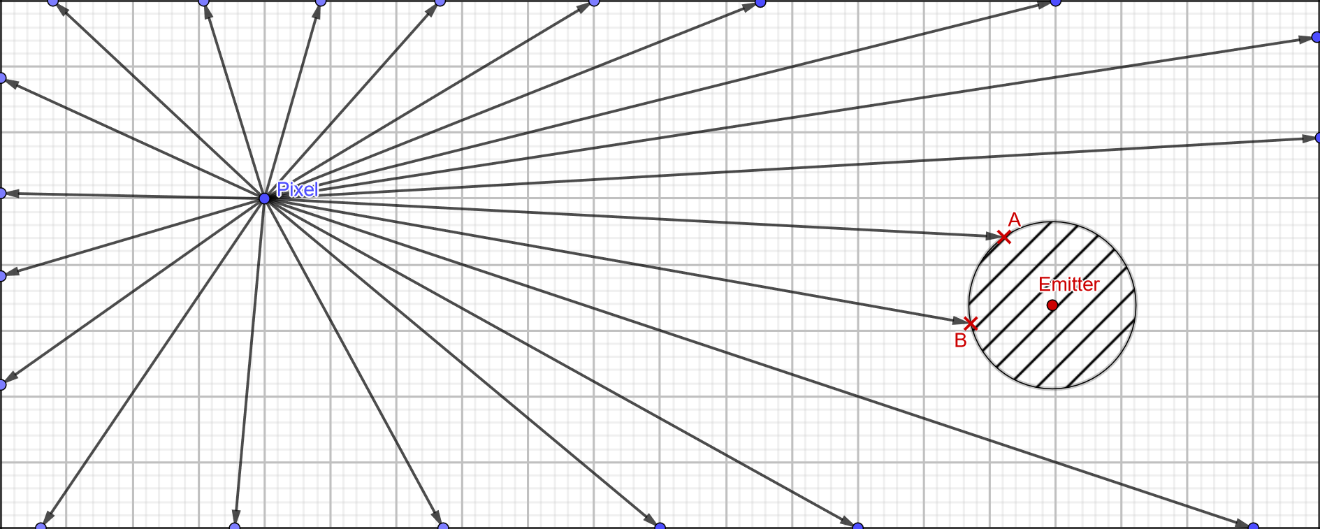
In our implementation we’re going to send a number of rays out from each pixel. These rays will travel until they hit a surface, and the emissive value of that surface will contribute to the total brightness value of that pixel. At a fundamental level it’s really that simple. What is complicated is how we determine what a surface is and when our ray has hit it, and how we get the emissive value from that pixel once we do.

A naive approach could be to sample each point on our ray in step size of one pixel. We’d need to sample every pixel to make sure we don’t jump past a surface. However, to do this would be exorbitantly expensive as a ray travelling from one side of our viewport to the other would potentially sample up to √(width²+height²) times. If only there was some way to encode the distance to the nearest surface in texture form that we could reference in our shader…

Distance Fields

A distance field is just that, a map where the value of each pixel is the distance from that pixel to the nearest surface. The reason this is useful for us is that instead of crawling along our ray one pixel at a time, we can sample the distance field at our current location and whatever value is returned, we know it is safe to advance exactly that far along the ray. This dramatically cuts down the amount of steps along our rays we need to do, in the best case we could jump straight from our ray origin to a surface, though in most cases it will still take a few steps (the worst case is that a ray is parallel and close to a surface, which means it will never reach the surface but can only step forward a small amount at a time).

There are two main ways to generate a distance field in a shader:

1. Naively sample in a radius around each pixel, and record the closest surface if one is found (or the max value if not). Very expensive.
2. Use the Jump Flooding algorithm (also see here) to generate a Voronoi Diagram, then convert that into a distance field.

Since #1 is completely impractical if we want the end result to run acceptably fast, we’re going to have to implement the Jump Flooding algorithm, then convert that Voronoi Diagram to a distance field. If you want more information on these then I recommend reading the links above, though don’t try to understand how the Jump Flooding algorithm works, it’s impossible and you might as well attribute it to magic.

Jump Flooding Part I - The Seed

(no that’s not a move in Super Mario Sunshine)

We need to seed the Jump Flooding algorithm with a copy of our emitter/occluder map, but each non-transparent pixel should store its own UV (a 2D vector between [0,0] and [1,1] that stores a position on a texture) in the RG component of the texture. To do this we’ll make a new Viewport with child TextureRect. This combo will be frequently used, the idea is the full-screen TextureRect draws the output of another viewport with our given shader, then it’s parent viewport stores that in its own texture ready to be drawn on another TextureRect. The whole render pipeline is primarily a daisy-chain of these Viewport + RenderTexture pairings.

On the RenderTexture, we set texture to a 1x1 image so there’s something to draw to, and set expand to true so it fills the whole viewport. Then we need to setup the material and shader that will actually convert the incoming emitter/occluder map to the seed for the Jump Flooding algorithm. Set material to be a new ShaderMaterial, and then set shader on that Material to a new Shader. You can then save that Shader for easy access later (I called mine VoronoiSeed.shader).

Now, we need to add some setup code below the previous setup code, in _ready():

func _ready():
   ...

   # setup our voronoi seed render texture.
   $VoronoiSeed.render_target_update_mode = Viewport.UPDATE_ALWAYS
   $VoronoiSeed.render_target_v_flip = true
   $VoronoiSeed.size = get_viewport().size
   $VoronoiSeed/Tex.rect_size = get_viewport().size
   $VoronoiSeed/Tex.material.set_shader_param("u_input_tex", $EmittersAndOccluders.get_texture())

   # set the screen texture to use the voronoi seed output.
   $Screen.texture = $VoronoiSeed.get_texture()

Finally, we need to add the GLSL (OpenGL Shader Language) code to the shader we just created.

shader_type canvas_item;

uniform sampler2D u_input_tex;

void fragment() 
{
   // for the voronoi seed texture we just store the UV of the pixel if the pixel is
   // part of an object (emissive or occluding), or black otherwise.
   vec4 scene_col = texture(u_input_tex, UV);
   COLOR = vec4(UV.x * scene_col.a, UV.y * scene_col.a, 0.0, 1.0);
}

Et voila, if everything went correctly (aka I didn’t forget any steps when writing this up) you should have something that looks like this:

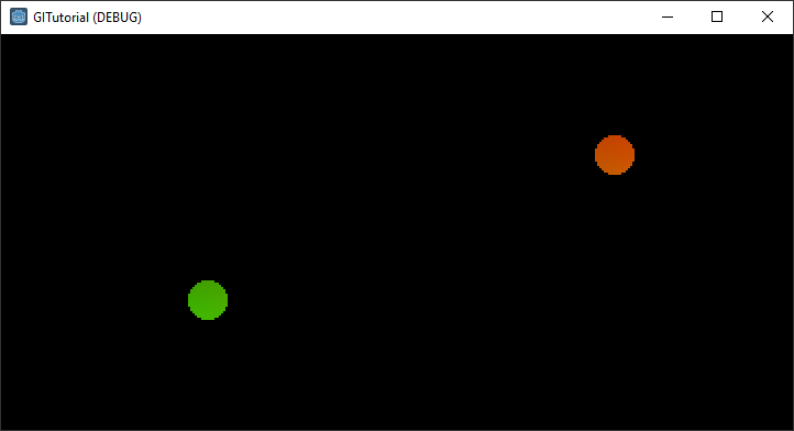
UV.x is represented on the red channel, so the sprite to the right appears red, and vice-versa.

Jump Flooding Part II - Multipass

Lets implement the actual Jump Flooding algorithm. Like I said before, I don’t know how this works, and you don’t need to either, suffice it to say that it does work and it’s actually very cheap (at least compared to our actual GI calculations that come later).

In short, we do a number of render passes, starting with the voronoi seed we created earlier, and ending with a full voronoi diagram. The number of iterations depends on the size of the buffer we’re working with. So, again we’ll set up a number of Viewport and TextureRect pairs (which I’ll call a render pass from now on) which we’ll daisy chain together, however since the amount of render passes is dynamic, we’ll create them programatically by duplicating a single render pass we set up in editor.

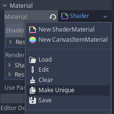
We create our initial jump flood render pass in the exact same way as our voronoi seed render pass, the only difference is that we point it to a brand new shader (empty for now). Be mindful if you duplicate the VoronoiSeed viewport, you’ll need to make the material unique or changes to the material on one viewport will be duplicated to the other. This has caught me out many times.

Again we add setup code to the _ready() function in the script attached to our root node, and we add _voronoi_passes[] which will keep track of our jump flooding render passes. There’s quite a lot going on here, but we’re basically just creating a bunch of render passes and setting up the correct shader uniforms (inputs).

var _voronoi_passes = []

func _ready():
   ...

   # setup our voronoi pass render texture.
   $JumpFloodPass.render_target_update_mode = Viewport.UPDATE_ALWAYS
   $JumpFloodPass.render_target_v_flip = true
   $JumpFloodPass.size = get_viewport().size
   $JumpFloodPass/Tex.rect_size = get_viewport().size

   # number of passes required is the log2 of the largest viewport dimension rounded up to the nearest power of 2.
   # i.e. 768x512 is log2(1024) == 10
   var passes = ceil(log(max(get_viewport().size.x, get_viewport().size.y)) / log(2.0))

   # iterate through each pass and set up the required render pass objects.
   for i in range(0, passes):

      # offset for each pass is half the previous one, starting at half the square resolution rounded up to nearest power 2.
      # i.e. for 768x512 we round up to 1024x1024 and the offset for the first pass is 512x512, then 256x256, etc. 
      var offset = pow(2, passes - i - 1)

      # on the first pass, use our existing render pass, on subsequent passes we duplicate the existing render pass.
      var render_pass
      if i == 0:
         render_pass = $JumpFloodPass
      else:
         render_pass = $JumpFloodPass.duplicate(0)
      add_child(render_pass)

      render_pass.get_child(0).material = render_pass.get_child(0).material.duplicate(0)
      _voronoi_passes.append(render_pass)

      # here we set the input texture for each pass, which is the previous pass, unless it's the first pass in which case it's
      # the seed texture.
      var input_texture = $VoronoiSeed.get_texture()
      if i > 0:
         input_texture = _voronoi_passes[i - 1].get_texture()

      # set size and shader uniforms for this pass.
      render_pass.set_size(get_viewport().size)
      render_pass.get_child(0).material.set_shader_param("u_level", i)
      render_pass.get_child(0).material.set_shader_param("u_max_steps", passes)
      render_pass.get_child(0).material.set_shader_param("u_offset", offset)
      render_pass.get_child(0).material.set_shader_param("u_input_tex", input_texture)

   # set the screen texture to use the final jump flooding pass output.
   $Screen.texture = _voronoi_passes[_voronoi_passes.size() - 1].get_texture()

Finally, we need to add the GLSL code which does most of the work.

shader_type canvas_item;

uniform sampler2D u_input_tex;
uniform float u_offset = 0.0; 
uniform float u_level = 0.0;
uniform float u_max_steps = 0.0;

void fragment() 
{
   float closest_dist = 9999999.9;
   vec2 closest_pos = vec2(0.0);

   // insert jump flooding algorithm here.
   for(float x = -1.0; x <= 1.0; x += 1.0)
   {
      for(float y = -1.0; y <= 1.0; y += 1.0)
      {
         vec2 voffset = UV;
         voffset += vec2(x, y) * SCREEN_PIXEL_SIZE * u_offset;

         vec2 pos = texture(u_input_tex, voffset).xy;
         float dist = distance(pos.xy, UV.xy);

         if(pos.x != 0.0 && pos.y != 0.0 && dist < closest_dist)
         {
            closest_dist = dist;
            closest_pos = pos;
         }
      }
   }
   COLOR = vec4(closest_pos, 0.0, 1.0);
}

Whew, that was a mouthful. It should look something like this when run:

This is a Voronoi Diagram, which is a map where each pixel stores the UV of the closest surface to it according to the seed input texture. It doesn’t look very exciting because our seed only contains two objects, so the Voronoi Diagram just carves the image into two regions with a line down the middle of our emitter and occluder. Play around with adding more sprites to the scene and see what Voronoi Diagrams you can create.

What’s more interesting to look at is the way a Voronoi Diagram is created over multiple passes:

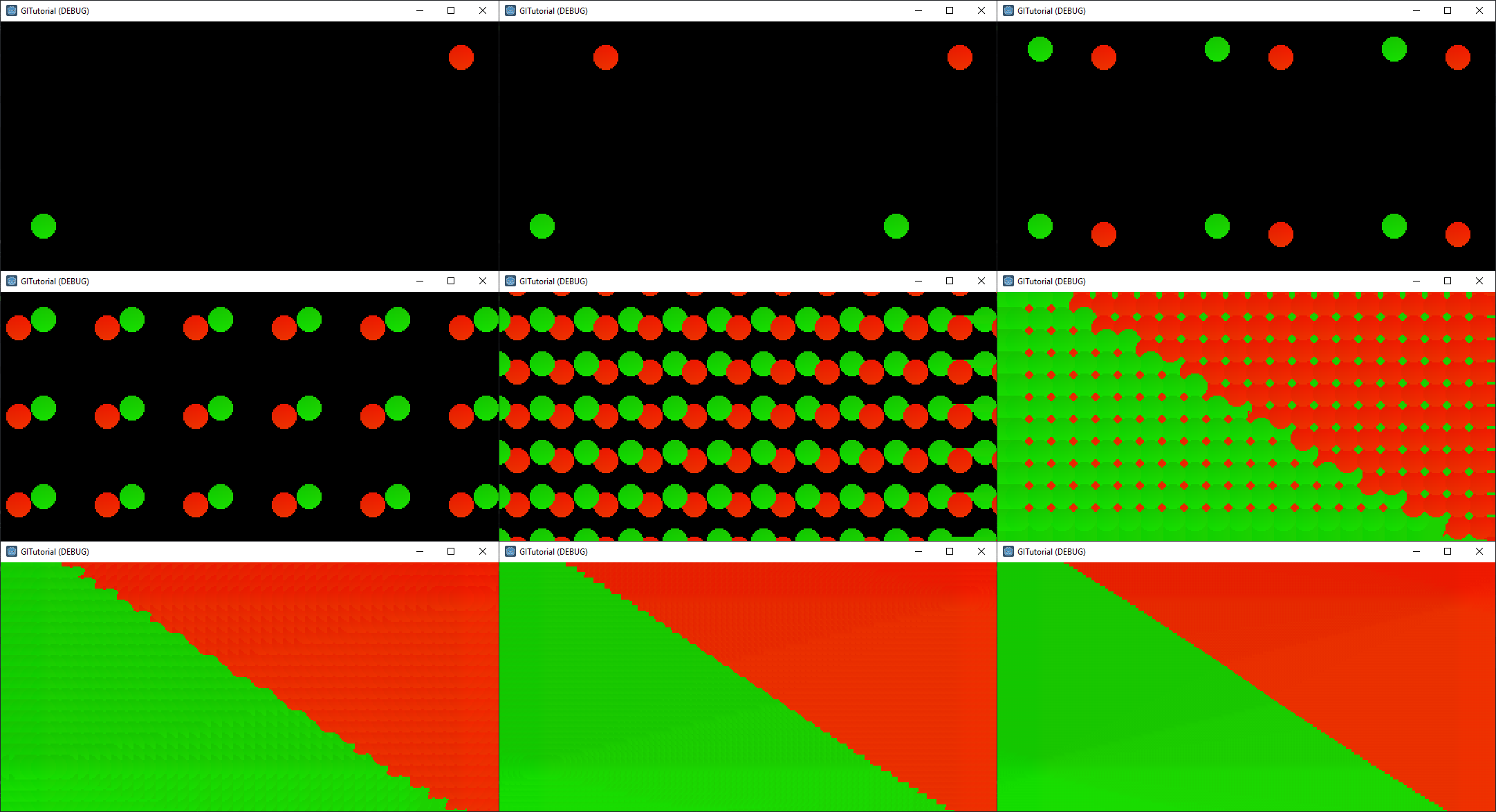
Creating The Distance Field

We’re finally ready to create a distance field! Thankfully, this is comparatively straight-forward compared to the Voronoi Diagram.

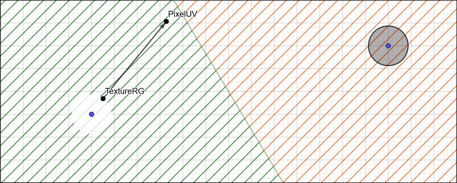
All we need to do, is for each pixel of the distance field, we sample the pixel at the same UV on the Voronoi Diagram and store the distance between it’s own UV (labeled PixelUV in the image below), and the UV stored in it’s RG channels (labeled as TextureRG below). We can then adjust this distance by some factor depending on what sort of precision/range trade-off we want, and that’s our distance field!

Create another render pass for the distance field, here’s what our full scene looks like right now:

Set it up as we’ve done before, the input texture is the final output from the jump flood render passes.

func _ready():
   ...
   # setup our distance field render texture.
   $DistanceField.transparent_bg = true
   $DistanceField.render_target_update_mode = Viewport.UPDATE_ALWAYS
   $DistanceField.render_target_v_flip = true
   $DistanceField.size = get_viewport().size
   $DistanceField/Tex.rect_size = get_viewport().size
   $DistanceField/Tex.material.set_shader_param("u_input_tex", _voronoi_passes[_voronoi_passes.size() - 1].get_texture())

   # set the screen texture to use the distance field output.
   $Screen.texture = $DistanceField.get_texture()

Finally, add the shader code. u_dist_mod can be left at 1.0 for now, basically it allows us to control the distance scaling, or how far from a surface before we report the max distance. Also worth noting is that the distance field is in UV space, that means a distance of 1.0 in the Y axis is the full height of the texture, and in X is the full width of the texture. This is an issue we’ll have to correct later.

shader_type canvas_item;

uniform sampler2D u_input_tex;
uniform float u_dist_mod = 1.0;

void fragment() 
{
   // input is the voronoi output which stores in each pixel the UVs of the closest surface.
   // here we simply take that value, calculate the distance between the closest surface and this
   // pixel, and return that distance. 
   vec4 tex = texture(u_input_tex, UV);
   float dist = distance(tex.xy, UV);
   float mapped = clamp(dist * u_dist_mod, 0.0, 1.0);
   COLOR = vec4(vec3(mapped), 1.0);
}

And we have something that looks like this:

It’s Time To Cast Some Rays

We now have everything we need to start writing our actual global illumination shader. The process will be something like this:

• For each pixel:
  • Cast X rays in a random direction.
  • For each ray:
    • Sample distance field.
    • If sample says we’ve hit a surface:
      • Sample the surface for emissive/colour data.
      • Increment the total emissive/colour value for this pixel.
      • Continue to next ray.
    • Else
      • Step forward by value returned by distance field sample.
    • Go back to ‘sample distance field’.
    • Continue stepping along the ray until we hit a surface, or the edge of the screen.
  • Normalise accumulated emissive/colour for number of rays.
  • Return pixel colour as emissive value * colour value.

Let’s break that down a bit.

Raycasting

At the core of most global illumination algorithms is random sampling of data to build up an increasingly accurate representation of the the ‘true’ solution as more samples are made. This is called the Monte Carlo method, and it relies on the natural tendency for randomness to converge on the correct answer given enough samples. In our case, the correct answer we’re converging upon is the solution to the rendering equation.

All the rays will have their origin at the current pixel. Their direction will be randomised using a sin wave crunched down enough that it gives a pseudorandom appearance, modified by the current pixel UV (so the random value is different per pixel) and time (so it’s different per frame).

Lets setup a new render pass, just like before, with a new shader that will contain all our global illumination shader code. At the bottom of our _ready() function, below the distance field setup code, setup the new GI render pass:

   # setup our distance field render texture.
   $GI.render_target_update_mode = Viewport.UPDATE_ALWAYS
   $GI.render_target_v_flip = true
   $GI.size = get_viewport().size
   $GI/Tex.rect_size = get_viewport().size
   $GI/Tex.material.set_shader_param("u_rays_per_pixel", 32)
   $GI/Tex.material.set_shader_param("u_distance_data", $DistanceField.get_texture())
   $GI/Tex.material.set_shader_param("u_scene_data", $EmittersAndOccluders.get_texture())
   $GI/Tex.material.set_shader_param("u_emission_multi", 1.0)
   $GI/Tex.material.set_shader_param("u_max_raymarch_steps", 128)

   # output our gi result to the screen
   $Screen.texture = $GI.get_texture();

We’ll then begin constructing our GI shader.

shader_type canvas_item;

// constants
uniform float PI = 3.141596;

// uniforms
uniform int u_rays_per_pixel = 32;
uniform sampler2D u_distance_data;
uniform sampler2D u_scene_data;
uniform float u_emission_multi = 1.0;
uniform int u_max_raymarch_steps = 128;
uniform float u_dist_mod = 1.0;

float random (vec2 st) 
{
   return fract(sin(dot(st.xy, vec2(12.9898,78.233))) * 43758.5453123);
}

void fragment() 
{
   float pixel_emis = 0.0;
   vec3 pixel_col = vec3(0.0);

   // convert from uv aspect to world aspect.
   vec2 uv = UV;
   float aspect = SCREEN_PIXEL_SIZE.y / SCREEN_PIXEL_SIZE.x;
   uv.x *= aspect;

   float rand2pi = random(UV * vec2(TIME, -TIME)) * 2.0 * PI;
   float golden_angle = PI * 0.7639320225; // magic number that gives us a good ray distribution.

   // cast our rays.
   for(int i = 0; i < u_rays_per_pixel; i++)
   {
      // get our ray dir by taking the random angle and adding golden_angle * ray number.
      float cur_angle = rand2pi + golden_angle * float(i);
      vec2 ray_dir = normalize(vec2(cos(cur_angle), sin(cur_angle)));
      vec2 ray_origin = uv;
      ...		

Hopefully most of this makes sense if you’ve been paying attention up until now. One possibly obscure part might be transforming the UV to world aspect ratio. We need to do this if our viewport is rectangular or our distances will be different depending on whether they’re biased towards the X or X axis. We’ll need to translate back to UV space before sampling any input textures.

Raymarching

We’ve sent our rays out, the next issue is how we determine when they hit the surface. This is the reason we went to the effort of creating a distance field, as it allows us to efficiently raymarch those rays to find any surface intersection point with as few steps as possible (since each step is a texture sample, and texture samples are generally expensive).

We’ll be using a specific raymarching method called sphere tracing (I guess circle tracing in 2D), where we adaptively step along a ray depending on the distance to the nearest surface, which we’ve calculated ahead of time in our distance field. Since we know no surface is closer than this distance, we can step forward that amount and then re-check the distance field. This is repeated until we hit a surface. It looks like this:

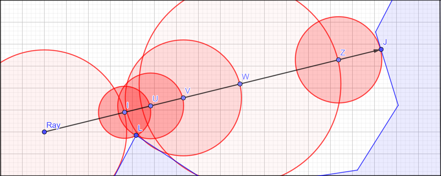
First we sample the distance field at the ray origin (Ray), which tells us the distance to the closest surface is at least the radius of the large circle around Ray, so we step forward to I. Again we check the DF, this time the closest surface is L so we step forward a shorter distance this time. We repeat this, taking steps of various sizes until we get to Z, and the next step takes us to J, which we know is a surface because sampling the DF now returns zero.

In practice, it looks like this:

bool raymarch(vec2 origin, vec2 dir, float aspect, out vec2 hit_pos)
{
   float current_dist = 0.0;
   for(int i = 0; i < u_max_raymarch_steps; i++)
   {
      vec2 sample_point = origin + dir * current_dist;
      sample_point.x /= aspect; // when we sample the distance field we need to convert back to uv space.

      // early exit if we hit the edge of the screen.
      if(sample_point.x > 1.0 || sample_point.x < 0.0 || sample_point.y > 1.0 || sample_point.y < 0.0)
         return false;

      float dist_to_surface = texture(u_distance_data, sample_point).r / u_dist_mod;

      // we've hit a surface if distance field returns 0 or close to 0 (due to our distance field using a 16-bit float
      // the precision isn't enough to just check against 0).
      if(dist_to_surface < 0.001f)
      {
         hit_pos = sample_point;
         return true;
      }

      // if we don't hit a surface, continue marching along the ray.
      current_dist += dist_to_surface;
   }
   return false;
}

At the bottom of _fragment():

void fragment() 
{
   ...
   vec2 hit_pos;
   bool hit = raymarch(ray_origin, ray_dir, aspect, hit_pos);
   if(hit)
   {
      ...
   }
}

There’s actually one more thing we should do to make this work correctly. You might remember that the distance field stores distances in UV space, which means that when we convert to screen space (i.e. pixels), the X and Y values will be skewed unless the screen is square. The easiest way to visualise this is if you imagine squishing your rectangular viewport square, so your perfectly circular sprites become elongated because the distances are skewed.

The result of this is that our raymarch steps will be either too long or too short, causing us to either step more than necessary, or worse step over surfaces completely causing visual glitches. There’s an easy way to fix this, and that’s to make our voronoi diagram viewport square, at a small cost of larger textures. We also need to do a bit of UV transforming to convert from our rectangular scene texture, to the square voronoi texture, and back again for the distance field.

For brevity we won’t go over the details here, if you’re following along you can resolve this by making your entire window square, or if your X resolution > Y resolution, you can ignore it knowing that you’re stepping a few more times than you need to.

Sampling The Surface And Putting It All Together

We’re almost done! Now that we know we’ve hit a surface, we can sample our scene texture at the hit location which will tell us the material properties of the surface. For now this is only emissive and colour, but we can add almost anything we’d like to improve the lighting simulation, such as 3D normal and height data, albedo, roughness, specular, etc.

Every ray hit will contribute that surface’s emissive and colour info to the current pixel, all we have to do it normalise those values by dividing by the number of rays.

First, lets add a function to our shader that can sample the scene data and return the emissive and colour info at that point:

void get_surface(vec2 uv, out float emissive, out vec3 colour)
{	
   vec4 emissive_data = texture(u_scene_data, uv);
   emissive = max(emissive_data.r, max(emissive_data.g, emissive_data.b)) * u_emission_multi;
   colour = emissive_data.rgb;
}

Next, we’ll update _fragment() so that when we hit a surface, we sample the surface data and add it to the accummulated total emissive and colour data for the current pixel:

...
if(hit)
{
   float mat_emissive;
   vec3 mat_colour;
   get_surface(hit_pos, mat_emissive, mat_colour);

   pixel_emis += mat_emissive;
   pixel_col += mat_colour;
}
...

Lastly, after we’ve accumulated the lighting data from all our rays, we’ll normalise the values and output the final pixel colour. One important note here is that we normalise pixel emissive on total number of rays, but pixel colour on the total accumulated emissive. This means the colour value maintains it’s magnitude (or brightness) regardless of how many rays were cast or surfaces hit. E.g. if we cast 32 rays and only 1 of them hit a red emitter, we want all of that red colour to contribute to the final pixel colour.

   ...
   pixel_col /= pixel_emis;
   pixel_emis /= float(u_rays_per_pixel);

   COLOR = vec4(pixel_emis * pixel_col, 1.0);
}

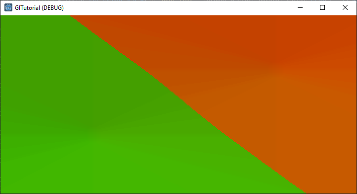
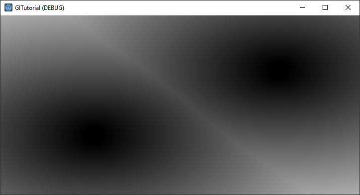
I feel like we’re more than deserving of some payoff after making it through all that. Hopefully everything compiles and hitting run will produce something that looks like this:

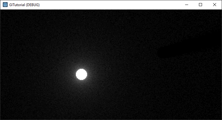
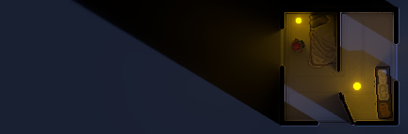
The Payoff

Ok, that’s maybe a little bit anti-climactic… It’s not very bright, you can’t even see the other occluder in the scene! However, don’t dispair dear reader, there’s a quick and easy resolution for this, and it comes in the form of four easily memorable letters. SRGB!

The problem is that the human eye is sensitive to low light conditions. We evolved this way so we could more easily find the light switch in the dark after stumbling in after a night of heavy drinking at The Winchester.

However, while working with colours in computer graphics we need to work with linear scales, so that maths does what we expect it to. In linear colour, the difference between 0.0 and 0.5 is the same as 0.5 to 1.0, whereas our eyes are much better at discerning differences in luminosity at the lower end of the scale than at the high end. SRGB aims to correct this, shifting more colour values down to the bottom end, effectively making dark values lighter.

All we need to do is create a new shader on our Screen TextureRect (the one that’s drawing our GI texture to the root viewport), and in that shader, run the GI texture through an SRGB function and output the final colour adjusted to SRGB colour space:

shader_type canvas_item;

uniform sampler2D u_GI_texture;

vec3 lin_to_srgb(vec4 color)
{
   vec3 x = color.rgb * 12.92;
   vec3 y = 1.055 * pow(clamp(color.rgb, 0.0, 1.0), vec3(0.4166667)) - 0.055;
   vec3 clr = color.rgb;
   clr.r = (color.r < 0.0031308) ? x.r : y.r;
   clr.g = (color.g < 0.0031308) ? x.g : y.g;
   clr.b = (color.b < 0.0031308) ? x.b : y.b;
   return clr.rgb;
}

void fragment() 
{
   vec4 GI = texture(u_GI_texture, UV);
   COLOR = vec4(lin_to_srgb(GI), 1.0);
}

Let’s try that again…

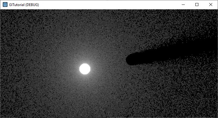
That’s a bit more like it! Notice how there’s now more range at the low-end of the brightness spectrum. Yes, it’s a lot noisier, since there’s more contrast in that lower range there is a bigger difference in brightness between, for example, a pixel where 2 rays hit an emitter and one where 3 hit an emitter. But that’s something we can improve on later with denoise filters and bounced light to fill in the gaps (or just whack up the number of rays!)

Lets add some more sprites, and use Godot’s modulate property to change the colours of our emitters. Remember that the sprites need to be children of the EmittersAndOccluders viewport in order to get included in the global illumination calculation.

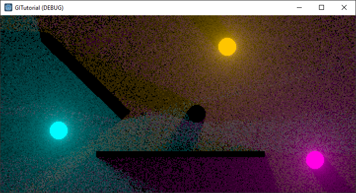
There’s lots of possibilities to continue toying with this. For example:

• Attach each sprite to a physics entity and have them bounce around everywhere.
• Increase the number of rays to reduce noise.
• Alter the contribution of an emissive surface based on the distance from the pixel, if you want to reduce or increase the emission range.
• Overlay the global illumination on an existing scene by multiplying it in the Screen shader.

That’s All For Now Folks

This is where we’ll stop for now, that was a lot of foundational knowledge and setup to get through, and this page is already far too long for any normal person to get through!

If you haven’t been following along and want to have a play with the completed project, or if you encountered problems along the way that you can’t seem to resolve, you can grab it from my GitHub.

I make no promises on when I will make the next part of the ‘2DGI in Godot’ series, but when it comes we’ll be looking at implementing bounced light for true global illumination (because to be honest, what we have right now isn’t any better than sprite based lighting). If you want a sneak-peak of that, there’s always my 2DGI in Godot demo source code to look at.

The best way to contact me with any questions is on Twitter, you can also leave a comment using the link below provided you have a GitHub account.